We interact with the number π (‘pi’) everyday. Due to its fundamental involvement with circles, π has found applications in virtually every industry, ranging from sports to designing power lines and everything in between. It would, then, seem absurd that a number that is seemingly so specific and universal can be estimated using just random numbers.

In this article, I shall first aim to explain how the value of π can be calculated using random numbers and I shall also provide a short Python code snippet that shows how this can be done and visualized by writing a simple program in just a few lines.

How Do We Calculate the Value of π Using Random Numbers?

I want to start by explaining what a Monte Carlo Simulation is. Monte Carlo Simulations can be thought of as computational algorithms that enable us to model probabilities that are difficult to calculate. This is done by using repeated random sampling to our advantage. With random sampling, the data we are using has no bias so we can simulate situations where the probabilities we obtain are close to the actual value. The more random data we use, the closer we get to the true value. Monte Carlo Simulations find their use in various fields, like Finance, Telecommunications and much more, however, we will not get into that in this article. In this article, we will analyze the use of a simple Monte Carlo Simulation to calculate the value of π (pi).

The entire basis of this method hinges on one of the most fundamental mathematical theorems that we all learn as children: the formula for the area of a circle.

For the purpose of this calculation, we must first take a graph, but only the first quadrant (the top-right section of a graph) is of interest to us. On this graph, we will create a square such that the length of each side of the square is 1 and the bottom left corner of the square lies at the origin. Essentially, this is constructed using line segments that lie on the x-axis, the y-axis, x=1 and y=1.

Now, we will plot a quarter-circle within the first quadrant of the graph. The radius of this circle will be 1 unit. This is formed with the equation x²+y²=1, 0≤x≤1, 0≤y≤1

Now, we must consider two sets of randomly generated numbers, x and y, that will represent the coordinates for a point on our graph. These random numbers will be generated such that they are a decimal number (floating point number) between 0 (inclusive) and 1 (exclusive): [0, 1).

This would then imply that any point generated in this manner will lie within the blue square, i.e. the probability that a point lies within the blue square is 1.

However, we must try and calculate the probability of a point lying within the red quarter-circle i.e. in the area shaded red here:

In order to check if a point lies within the red shaded region, we must check whether or not the point satisfies the condition: x²+y²≤1 since this inequality represents the shaded area within the constraints of 0≤x≤1, 0≤y≤1.

Since the red area represents the area of one-quarter of a circle, the area is represented by:

Logically, if we could generate points that follow the conditions mentioned earlier, we could obtain the value of π.

One key observation is that the calculated value of π gets closer to the true value if we increase the number of points under consideration since a larger number of points brings us closer to a truly random situation.

Visualizing the Process

We used a random number generator to generate a set of 10 random values of x and 10 corresponding values of y such that 0≤x≤1and 0≤y≤1.

Next, these points were plotted on the graph.

The green points represent points that are within the red quarter-circle and the red points represent points that lie outside it. We can see that 8 out of the 10 points lie within the red circle.

Although this is not the exact value of π, for a set of just 10 points, it is remarkably close. In order to see how the value becomes closer to the true value of π with an increase in the number of points we take into consideration, we must write a few lines of code.

Code to Calculate the Value of Using Random Numbers

The code that one needs to write in order to perform this operation is extremely simple. The following snippet in Python that can be used to visualize the points that we are plotting and also calculate the value of π as described above:

import numpy as npimport matplotlib.pyplot as plt%matplotlib inline#Defining the lines of the square:horiz = np.array(range(100))/100.0y_1 = np.ones(100)plt.plot(horiz , y_1, 'b')vert = np.array(range(100))/100.0x_1 = np.ones(100)plt.plot(x_1 , vert, 'b')#Plotting the random points:import randominside = 0i=1n=int(input("Enter the total number of points: "))while (i<=n): x = random.random() y = random.random() if ((x**2)+(y**2))<=1: inside+=1 plt.plot(x , y , 'go') else: plt.plot(x , y , 'ro') i+=1pi=(4*inside)/nprint ("The value of pi is:")print(pi)plt.show()

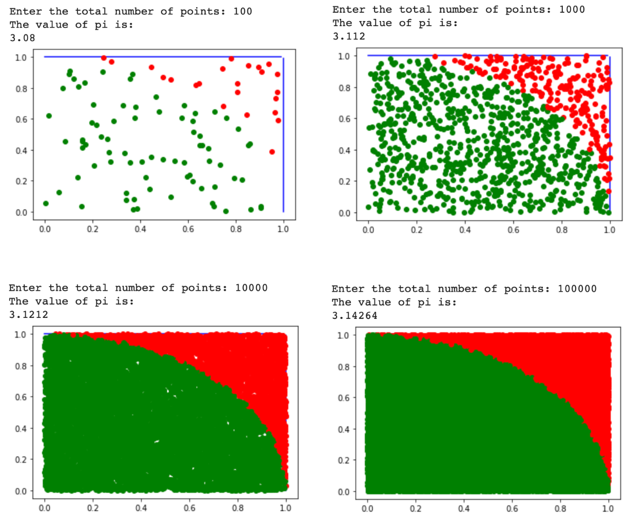
This code was executed for 100, 1000, 10000 and 100000 random data points and these were the results:

As can be seen, with the increase in the total number of datapoints, the separation between the red and green points begins to look more and more like a perfectly drawn quarter-circle. This correlates with the general trend of the increase in how close our calculated value of π is to the actual value with an increase in the number of datapoints.

Concluding Remarks

While it does seem somewhat strange that a number as specific and widely used as π can be calculated using a set of randomly generated numbers, I choose to look at this in a slightly more philosophical sense. Perhaps, this is an indication that the universe as a whole exists in a state of randomness (entropy) and the path to success is for us to identify the unifying truths about the universe. The value of π can be thought of as one such universal truth that has helped increase the degree of “order” that we can perceive in the universe around us.